Biodiversity metrics and metabarcoding
2/2/24
Not all the PCR have the same number of reads
Despite all standardization efforts

Is it related to the amount of DNA in the extract ?
What do the reading numbers per PCR mean?
Rarefying read count (2)
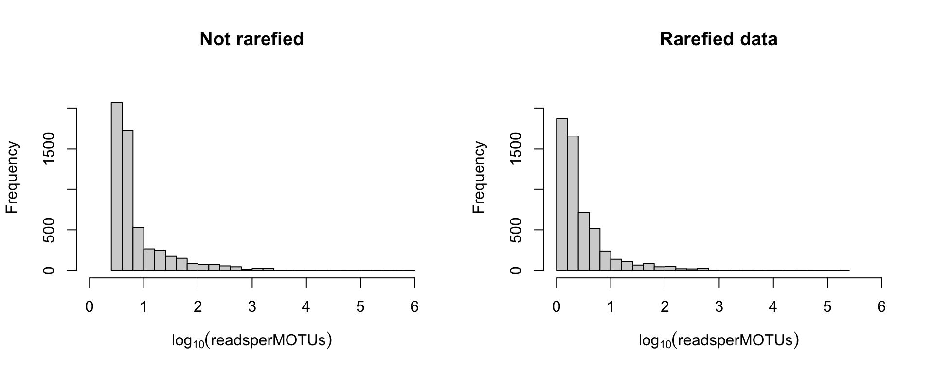
Rarefying read count (4)

The MOTUs removed by rarefaction were at most occurring 20 times
The MOTUs kept by rarefaction were at least occurring 2 times
Why rarefying ?

Increasing the number of reads just increase the description of the subpart of the PCR you have sequenced.
The different types of diversity

Whittaker (2010)
\(\alpha\text{-diversity}\) : Mean diversity per site (\(species/site\))
\(\gamma\text{-diversity}\) : Regional biodiversity (\(species/region\))
\(\beta\text{-diversity}\) : \(\beta = \frac{\gamma}{\alpha}\) (\(sites/region\))
Which is th most diverse environment ?

| A | B | C | D | E | F | G | |
|---|---|---|---|---|---|---|---|
| Environment.1 | 0.25 | 0.25 | 0.25 | 0.25 | 0.00 | 0.00 | 0.00 |
| Environment.2 | 0.55 | 0.07 | 0.02 | 0.17 | 0.07 | 0.07 | 0.03 |
Richness
The actual number of species present in your environement whatever their aboundances
| S | |
|---|---|
| Environment.1 | 4 |
| Environment.2 | 7 |
Gini-Simpson’s index
The Simpson’s index is the probability of having the same species twice when you randomly select two specimens.
\[
\lambda =\sum _{i=1}^{S}p_{i}^{2}
\]
\(\lambda\) decrease when complexity of your ecosystem increase.
Gini-Simpson’s index defined as \(1-\lambda\) increase with diversity
| Gini.Simpson | |
|---|---|
| Environment.1 | 0.7500 |
| Environment.2 | 0.6526 |
Shannon entropy
Shannon entropy is based on information theory:
if \(A\) is a community where every species are equally represented then \[ H(A) = \log|A| \]
| Shannon.index | |
|---|---|
| Environment.1 | 1.386294 |
| Environment.2 | 1.371925 |
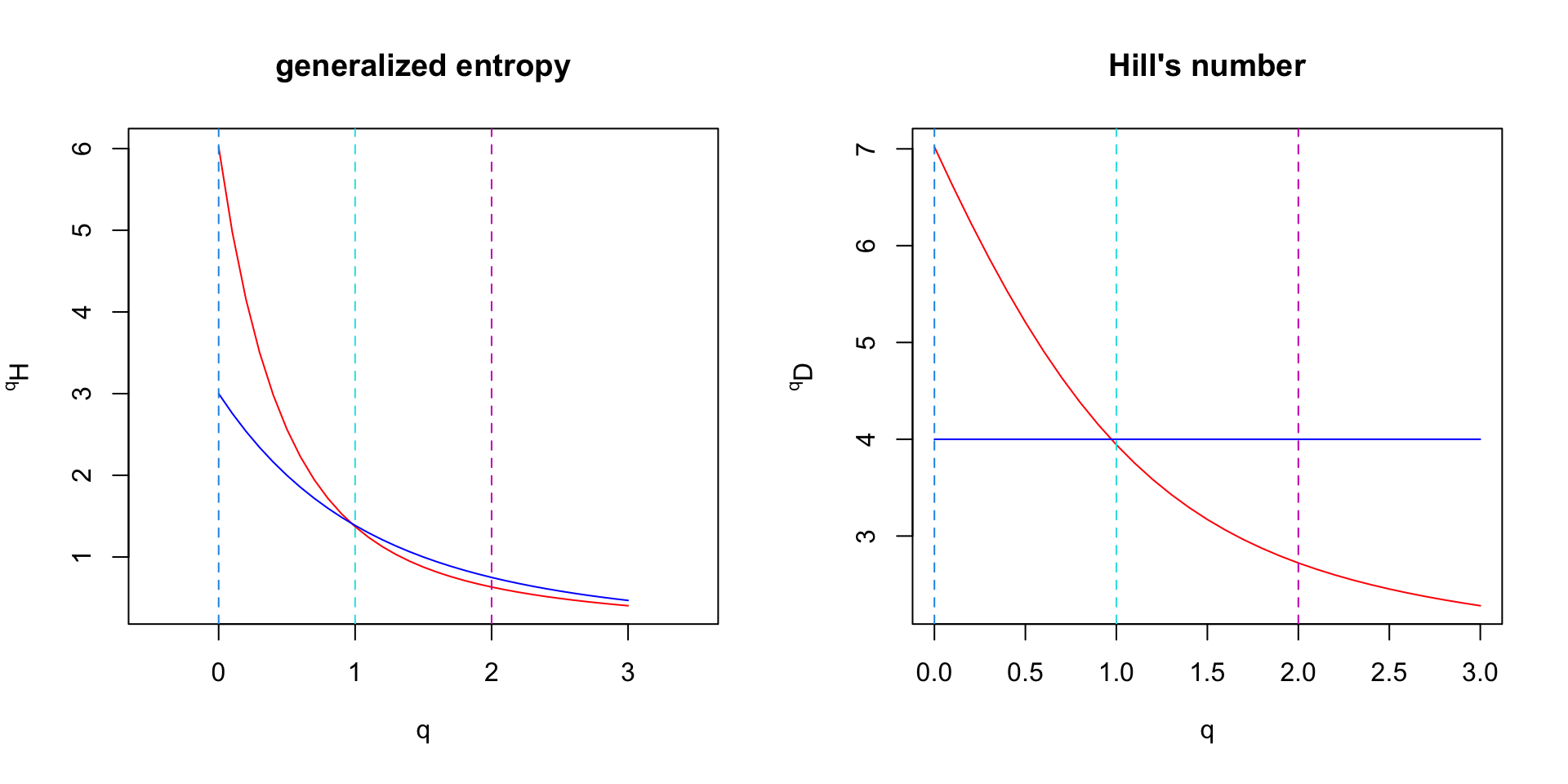
Hill’s number
As : \[
H(A) = \log|A| \;\Rightarrow\; ^1D = e^{H(A)}
\]
where \(^1D\) is the theoretical number of species in a evenly distributed community that would have the same Shannon’s entropy than ours.
| Hill.Numbers | |
|---|---|
| Environment.1 | 4.000000 |
| Environment.2 | 3.942933 |
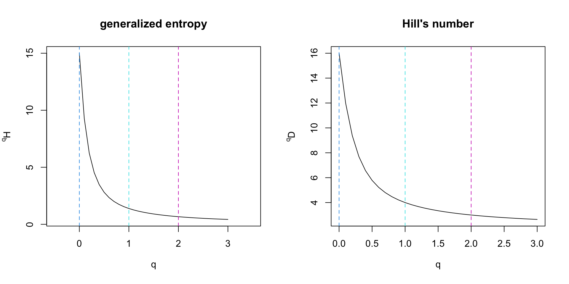
Impact of \(q\) on the log_q function
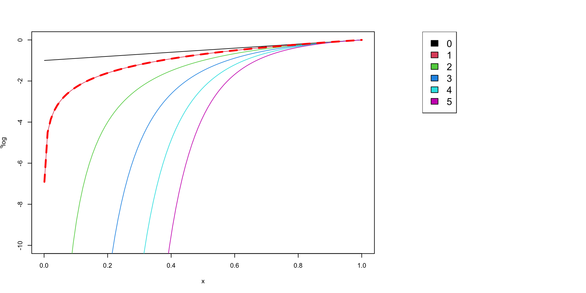
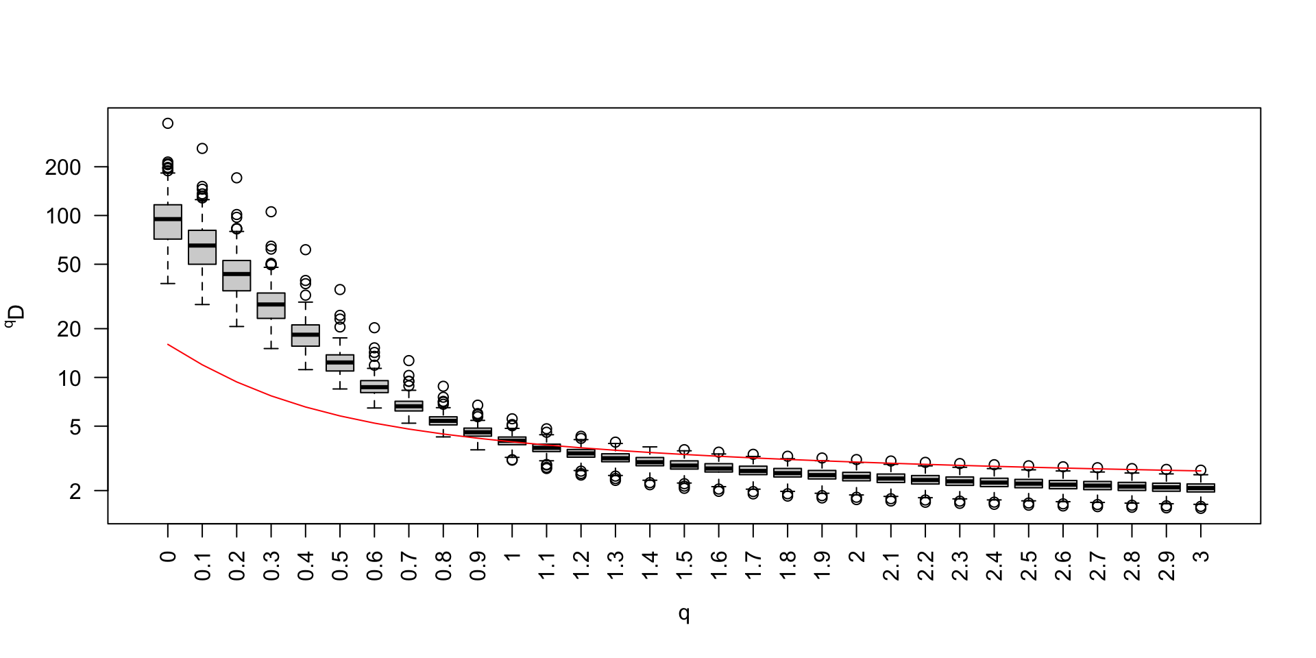
Biodiversity spectrum (2)
Biodiversity spectrum of the mock community
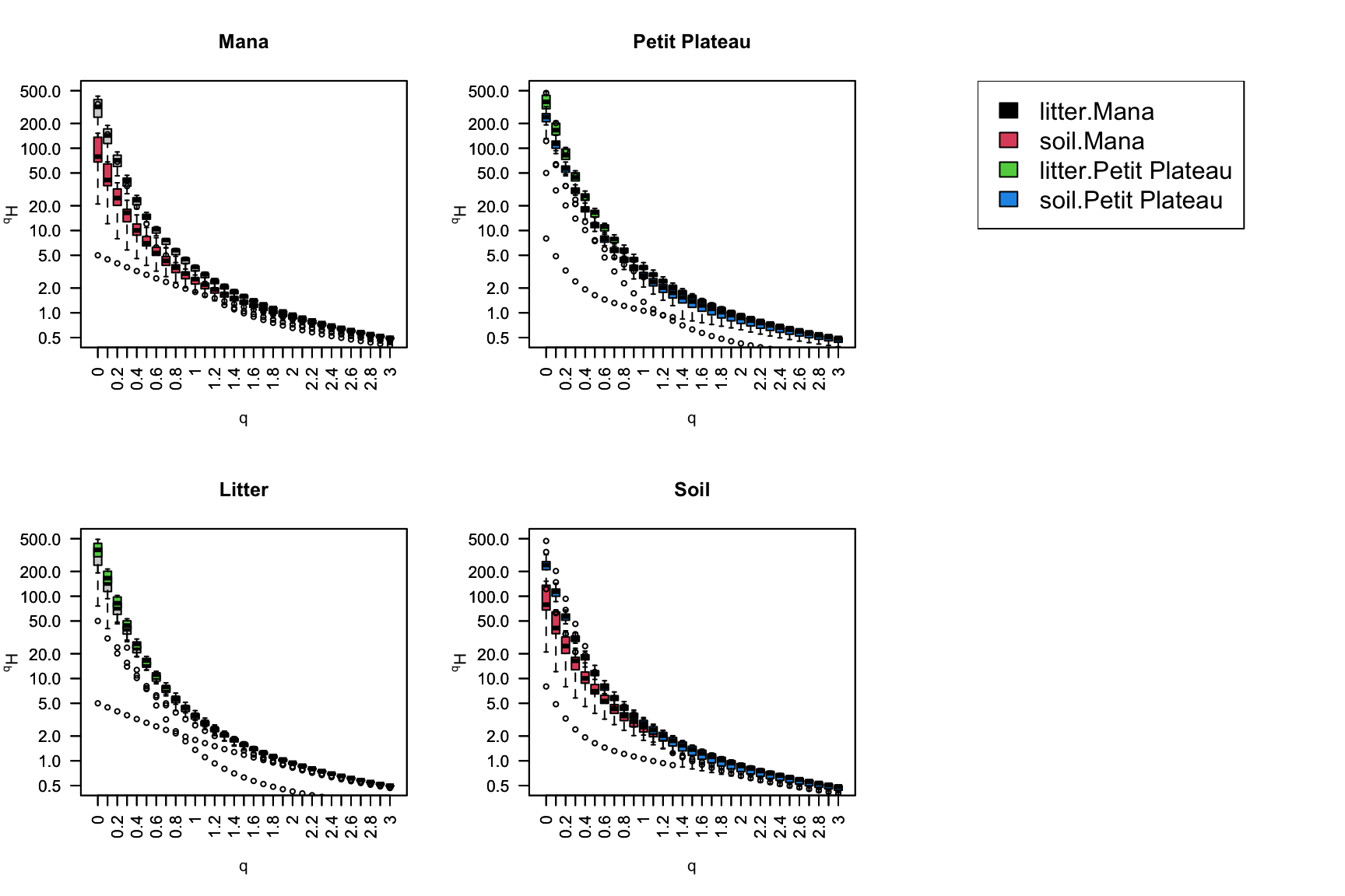
Biodiversity spectrum and metabarcoding (1)
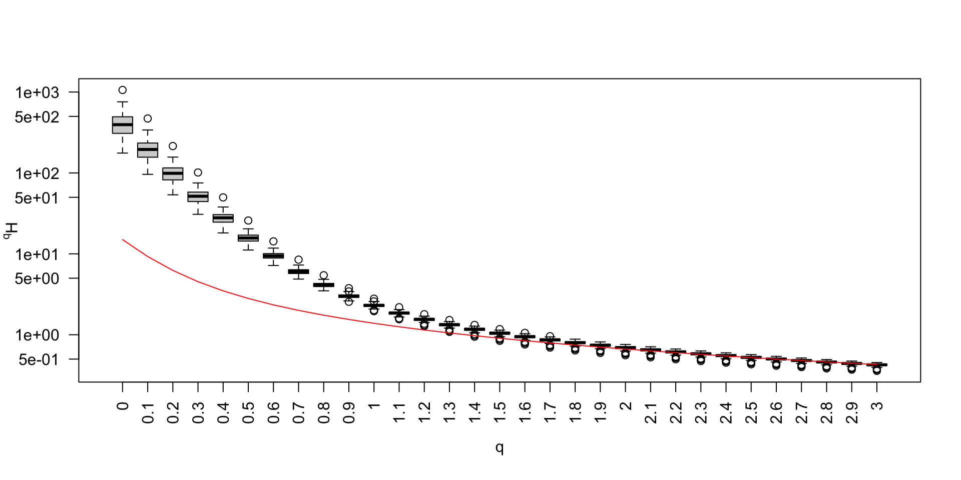
Biodiversity spectrum and metabarcoding (2)
Biodiversity spectrum and metabarcoding (3)
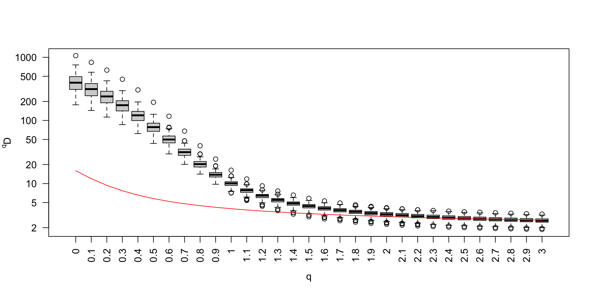
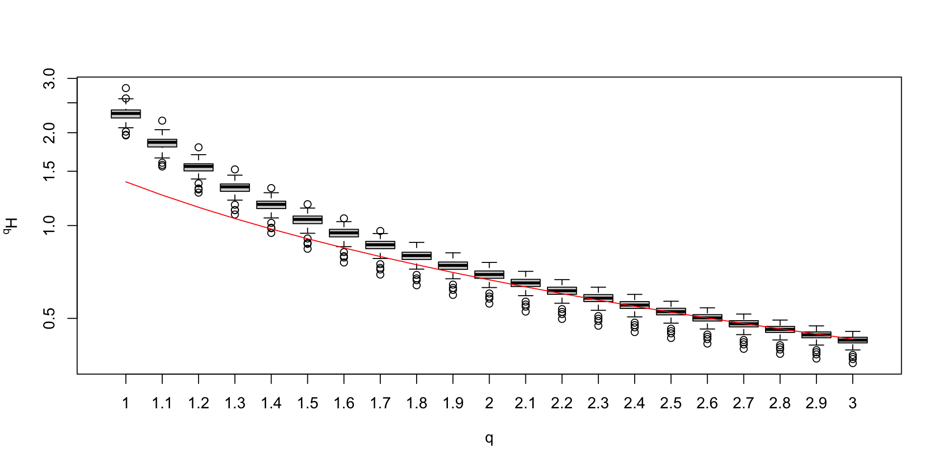
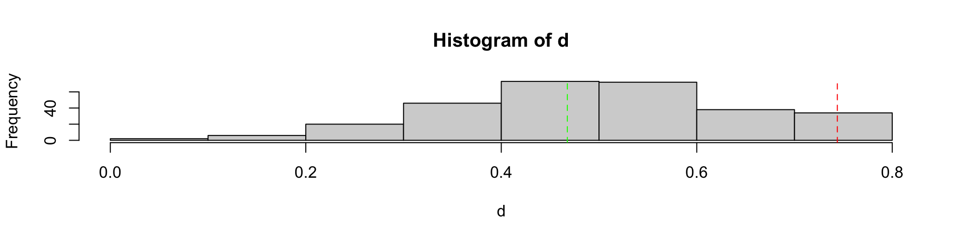
Impact of data cleaning on \(\alpha\)-diversity (2)

Impact of data cleaning on \(\alpha\)-diversity (3)
Metrics or distances

A metric is a dissimilarity index verifying the subadditivity also named triangle inequality
\[ \begin{align} d(A,B) \geqslant& 0 \\ d(A,B) =& \;d(B,A) \\ d(A,B) =& \;0 \iff A = B \\ d(A,B) \leqslant& \;d(A,C) + d(C,B) \end{align} \]
Some metrics

Computing
\[ \begin{align} d_e =& \sqrt{(x_A - x_B)^2 + (y_A - y_B)^2} \\ d_m =& |x_A - x_B| + |y_A - y_B| \\ d_c =& \max(|x_A - x_B| , |y_A - y_B|) \\ \end{align} \]
Metrics and ultrametrics

Metric
\[ d(x,z)\leqslant d(x,y)+d(y,z) \]
Ultrametric
\[ d(x,z)\leq \max(d(x,y),d(y,z)) \]
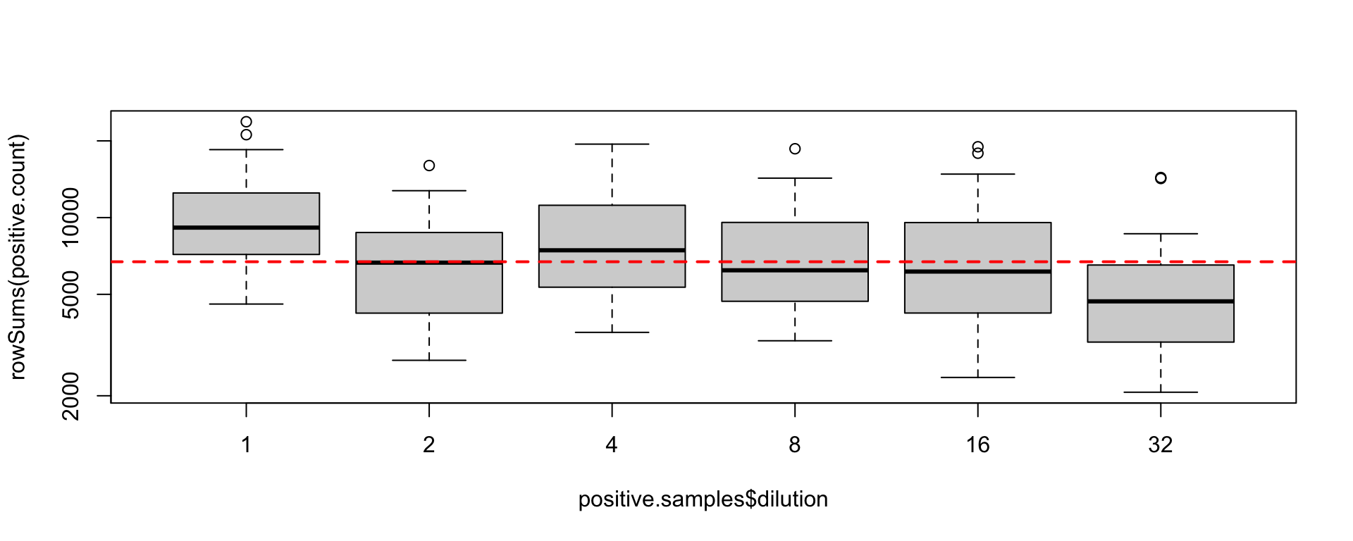
Clean out bad PCR cycle 1
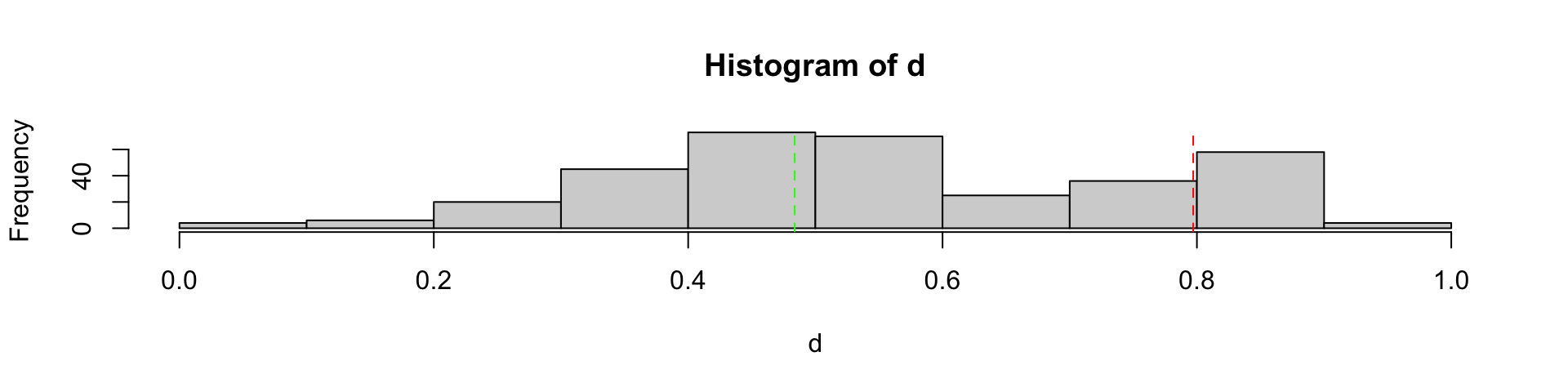
Clean out bad PCR cycle 2
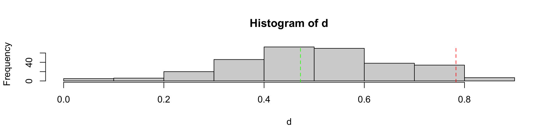
Clean out bad PCR cycle 3
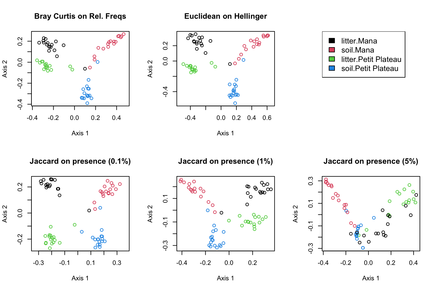
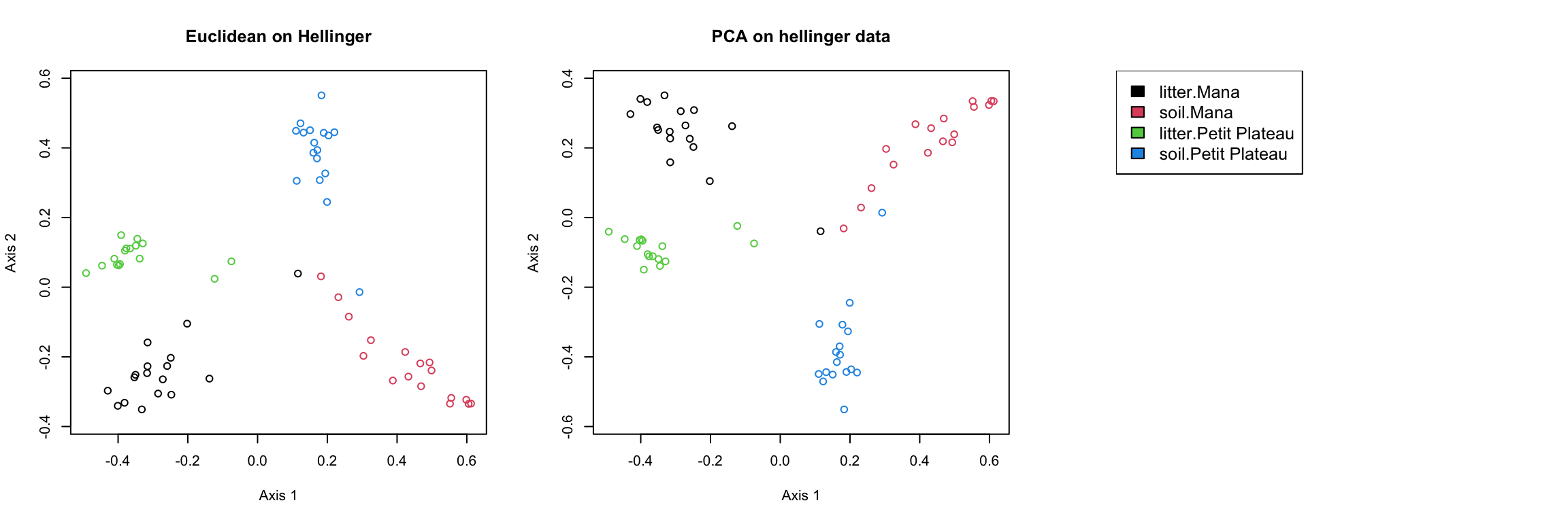
Euclidean distance on Hellinger transformation


Principale coordinate analysis (2)
Principale composante analysis
Comparing diversity of the environments